Threshold Weighted Continuous Ranked Probability Score (twCRPS) for ensembles#
twCRPS can be used to evaluate ensembles while emphasising extremes or a range of important thresholds. Sometimes CRPS may mask performance around extremes and it may be desirable to use a threshold weighted score such as twCRPS. If you haven’t done so, we recommend working through the CRPS for forecasts expressed as CDFs and CRPS for ensemble forecasts tutorials before working through this tutorial. Note that the crps_cdf function
has threshold weighting built into it, but the crps_for_ensemble does not. This tutorial will demonstrate how to calculate a threshold weighted CRPS for ensembles.
Overview and graphical illustration of twCRPS#
We will begin by illustrating how the twCRPS for ensembles is calculated, first by defining the equation and then with a graphical representation. The emperical twCRPS for ensembles is defined as
where - \(M\) is the number of ensemble members, - \(y\) is the observation, - \(x_m\) is the forecast of a single ensemble member, - \(x_j\) is also the forecast of a single ensemble member, and - \(v\) is a ‘chaining function’.
The chaining function \(v\) is an anti-derivative of the threshold weight function \(w\), which is a non-negative function that assigns a weight to each threshold value.
For example, if we wanted to assign a threshold weight of 1 to thresholds above threshold \(t\) and a threshold weight of 0 to thresholds below \(t\), our threshold weight function would be \(w(x) = \mathbb{1}{(x > t)}\), where \(\mathbb{1}\) is the indicator function which returns a value of 1 if the condition is true and 0 otherwise. A chaining function would then be \(v(x) = \text{max}(x, t)\).
Let’s now visualise what the weighting and chaining functions if we were to set \(t=25\) for weighting an upper tail. Let’s assume that we are working with rainfall data with mm as the units.
[1]:
import plotly.graph_objects as go
import numpy as np
from plotly.subplots import make_subplots

x = np.linspace(0, 100, 400)
t = 25

# Calculate w(x)
w_x = np.where(x > t, 1, 0)
# Calculate v(x)
v_x = np.maximum(x, t)

fig = make_subplots(
    rows=2,
    cols=1,
    subplot_titles=("Weight function: w(x) = 1(x>t)", "Chaining function: v(x) = max(x, t)"),
    vertical_spacing=0.15,
)
fig.add_trace(go.Scatter(x=x, y=w_x, mode="lines", name="w(x) = 1(x>t)", showlegend=False), row=1, col=1)
fig.add_trace(go.Scatter(x=x, y=v_x, mode="lines", name="v(x) = max(x, t)", showlegend=False), row=2, col=1)

fig.update_layout(
    xaxis_title="x (mm)",
    yaxis_title="w",
    xaxis2_title="x (mm)",
    yaxis2_title="v",
    showlegend=True,
    width=600,
    height=600,
    margin=dict(l=20, r=20, t=40, b=60),
)
fig.show()
Now let’s produce an illustration of what the difference between CRPS and twCRPS would look like.
We will visualise the CDF of an ensemble with 50 ensemble members against an observation of 50mm
[2]:
np.random.seed(100)
# Produce CDF from ensemble
data = np.random.uniform(0, 70, 50)
sorted_data = np.sort(data)
cdf = np.arange(1, len(sorted_data) + 1) / len(sorted_data)

# Round the value closest to 25 to exactly 25 to make plot line up nicely
index_closest_to_25 = np.argmin(np.abs(sorted_data - 25))
sorted_data[index_closest_to_25] = 25

# Tidy up the beginning of the CDF
sorted_data = np.insert(sorted_data, 0, 0)
cdf = np.insert(cdf, 0, 0)

# Create the observation
x = np.linspace(0, 71, 4000)
obs_cdf = np.where(x > 50, 1, 0)

fig = go.Figure()
fig.add_trace(
    go.Scatter(
        x=sorted_data[np.where(sorted_data >= 25)],
        y=cdf[np.where(sorted_data >= 25)],
        mode="lines",
        name="Forecast CDF",
        line_shape="hv",
        showlegend=False,
    )
)
fig.add_trace(
    go.Scatter(
        x=x[np.where(x >= 25)],
        y=obs_cdf[np.where(x >= 25)],
        mode="lines",
        name="Observed CDF",
        fill="tonexty",
        fillcolor="rgba(176,224,230, 0.7)",
        showlegend=False,
    )
)
fig.add_trace(
    go.Scatter(x=sorted_data, y=cdf, mode="lines", name="Forecast CDF", line_shape="hv", line=dict(color="blue"))
)
fig.add_trace(go.Scatter(x=x, y=obs_cdf, mode="lines", name="Observed CDF", line=dict(color="red")))

fig.update_layout(
    title="Graphical illustration of twCRPS",
    yaxis_title="Probability of non-exceedance",
    xaxis_title="x (mm)",
    showlegend=True,
    width=600,
    height=600,
    margin=dict(l=20, r=20, t=40, b=60),
    legend=dict(x=0.01, y=0.99, xanchor="left", yanchor="top"),
)


fig.show()
The shaded area between the two lines equals the twCRPS for \(w(x) = \mathbb{1}{(x > 25)}\) and \(v(x) = \text{max}(x, 25)\). It measures predictive performance for decision thresholds above 25mm.
Calculating twCRPS with scores#
Let’s get forecasts from the ECMWF IFS ensemble and from the Neural GCM which is a general circulation model “that combines a differentiable solver for atmospheric dynamics with machine-learning components”. We will evaluate the forecasts against ERA5 data. All data is retrieved from WeatherBench2 and is regridded to a 1.5 degree grid.
While pure machine learning (data driven) models, or hybrid models that combine physical modelling with machine learning have been shown to be quite good when evaluated using standard verificaiton statistics, it may be interesting to see how well the perform at predicting extremes. We can use twCRPS to measure how Neural GCM compares to the ECWMF IFS ensemble in predicting extremes or a range of key decision thresholds.
It may take around 30 seconds to establish a connection with the cloud storage when running for the first time.
We will demonstrate three different functions: 1. scores.probability.tail_tw_crps_for_ensemble for emphasising performance for an upper or lower tail (e.g., for extremes) 2. scores.probability.interval_tw_crps_for_ensemble for emphasising performance across an interval of decision thresholds 3. scores.probability.tw_crps_for_ensemble for emphasising performance based on custom weights
[3]:
import xarray as xr
import pandas as pd
from scores.probability import tail_tw_crps_for_ensemble, interval_tw_crps_for_ensemble, tw_crps_for_ensemble
from scores.functions import create_latitude_weights
from scores.processing import broadcast_and_match_nan

# You can view the documentation for the function by running the following

# help(tw_crps_for_ensemble)
# help(interval_tw_crps_for_ensemble)
# help(tail_tw_crps_for_ensemble)
[4]:
ifs_ens = xr.open_zarr("gs://weatherbench2/datasets/ifs_ens/2018-2022-240x121_equiangular_with_poles_conservative.zarr")
neural_gcm = xr.open_zarr(
    "gs://weatherbench2/datasets/neuralgcm_ens/2020-240x121_equiangular_with_poles_conservative.zarr"
)
era5 = xr.open_zarr(
    "gs://weatherbench2/datasets/era5/1959-2023_01_10-6h-240x121_equiangular_with_poles_conservative.zarr"
)
Example 1. 850hPa wind speed - focusing on gales or stronger#
Suppose you are hot air ballooning and you want to compare the performance of two ensembles that produce wind speed forecasts at 850hPa at a lead time of 48 hours, but you only care about the performance for decision thresholds above 17.2 m/s (the threshold for gale force winds). We will just pull down the first week of data (with 6 hourly timesteps) in January 2020 which will should take under a minute unless you have a very slow internet connection.
We will use the scores.probability.tail_tw_crps_for_ensemble function.
[5]:
lead_time = pd.Timedelta("2d")
ifs_ens_wind = ifs_ens.wind_speed.sel(
    level=850, time=slice("2020-03-01T00:00:00", "2020-03-07T00:00:00"), prediction_timedelta=lead_time
).compute()
neural_gcm_wind = neural_gcm.wind_speed.sel(
    level=850, time=slice("2020-03-01T00:00:00", "2020-03-07T00:00:00"), prediction_timedelta=lead_time
).compute()
era5_wind = era5.wind_speed.sel(level=850, time=slice("2020-03-03T00:00:00", "2020-03-09T00:00:00")).compute()
[6]:
# Update the time coords in the forecast to match up to the observations
ifs_ens_wind = ifs_ens_wind.assign_coords({"time": ifs_ens_wind.time + lead_time})
neural_gcm_wind = neural_gcm_wind.assign_coords({"time": neural_gcm_wind.time + lead_time})

# Rename the ensemble member dimension to number to match the IFS naming
neural_gcm_wind = neural_gcm_wind.rename({"realization": "number"})

# Match any missing data between the two forecasts that we are comparing
ifs_ens_wind, neural_gcm_wind = broadcast_and_match_nan(ifs_ens_wind, neural_gcm_wind)
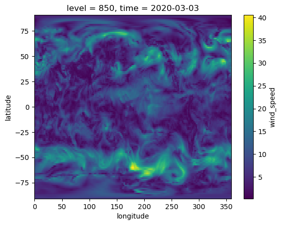
Let’s visualise the observations for the first timestep
[7]:
era5_wind.T.sel(time="2020-03-03T00:00:00").plot()
[7]:
<matplotlib.collections.QuadMesh at 0x14c0d3d70>
Now, let’s calculate twCRPS focusing on performance above the decision threshold 17.2 m/s for the two models.
[8]:
# First create weights for weighting the grid cells by latitude when we calculate the mean twCRPS. These differ from the threshold weights
lat_weights = create_latitude_weights(ifs_ens_wind.latitude)
tail_tw_crps_for_ensemble(
    ifs_ens_wind, era5_wind, threshold=17.2, tail="upper", ensemble_member_dim="number", weights=lat_weights
)
[8]:
<xarray.DataArray ()>
array(0.06075118)
Coordinates:
    level                 int32 850
prediction_timedelta timedelta64[ns] 2 days[9]:
tail_tw_crps_for_ensemble(
    neural_gcm_wind, era5_wind, threshold=17.2, tail="upper", ensemble_member_dim="number", weights=lat_weights
)
[9]:
<xarray.DataArray ()>
array(0.05780117)
Coordinates:
    level                 int64 850
prediction_timedelta timedelta64[ns] 2 daysThe twCRPS was lower (better) for the Neural GCM than ECMWF IFS ensemble for this week of data.
Example 2. 850hPa temperatures - focusing on an interval of decision thresholds#
Now, suppose that we want to understand which model produces better forecasts of temperatures for decision thresholds between -20 degrees C and -10 degrees C where aircraft icing is most likely to occur. That is, we want to assign a weight of 1 to decision thresholds between -20 and -10, and a weight of 0 elsewhere. This should also take under a minute to download the data.
We will use the scores.probability.interval_tw_crps_for_ensemble function. First, let’s visualise the chaining and weighting functions.
[10]:
x = np.linspace(-30, 10, 400)
a = -20
b = -10

# Calculate w(x)
w_x = np.zeros_like(x)
w_x[(x >= -20) & (x <= -10)] = 1

# Calculate v(x)
v_x = np.minimum(np.maximum(x, a), b)

fig = make_subplots(
    rows=2,
    cols=1,
    subplot_titles=("Weight function: w(x) = 1(a < x < b)", "Chaining function: v(x) = min(max(x, a), b)"),
    vertical_spacing=0.15,
)
fig.add_trace(go.Scatter(x=x, y=w_x, mode="lines", name="w(x) = 1(x>t)", showlegend=False), row=1, col=1)
fig.add_trace(go.Scatter(x=x, y=v_x, mode="lines", name="v(x) = min(max(x, a), b)", showlegend=False), row=2, col=1)

fig.update_layout(
    xaxis_title="x (mm)",
    yaxis_title="w",
    xaxis2_title="x (mm)",
    yaxis2_title="v",
    showlegend=True,
    width=600,
    height=600,
    margin=dict(l=20, r=20, t=40, b=60),
)
fig.show()
[11]:
lead_time = pd.Timedelta("2d")
ifs_ens_temp = ifs_ens.temperature.sel(
    level=850, time=slice("2020-03-01T00:00:00", "2020-03-07T00:00:00"), prediction_timedelta=lead_time
).compute()
neural_gcm_temp = neural_gcm.temperature.sel(
    level=850, time=slice("2020-03-01T00:00:00", "2020-03-07T00:00:00"), prediction_timedelta=lead_time
).compute()
era5_temp = era5.temperature.sel(level=850, time=slice("2020-03-03T00:00:00", "2020-03-09T00:00:00")).compute()
[12]:
# Update the time coords in the forecast to match up to the observations
ifs_ens_temp = ifs_ens_temp.assign_coords({"time": ifs_ens_temp.time + lead_time})
neural_gcm_temp = neural_gcm_temp.assign_coords({"time": neural_gcm_temp.time + lead_time})

# Rename the ensemble member dimension to number to match the IFS naming
neural_gcm_temp = neural_gcm_temp.rename({"realization": "number"})

# Match any missing data between the two forecasts that we are comparing
ifs_ens_wind, neural_gcm_wind = broadcast_and_match_nan(ifs_ens_wind, neural_gcm_wind)

# Convert the temperature to Celsius
ifs_ens_temp -= 273.15
neural_gcm_temp -= 273.15
era5_temp -= 273.15
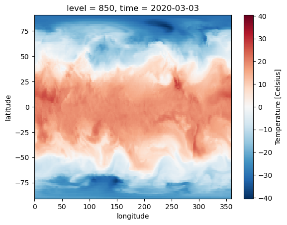
Let’s visualise the observations for the first timestep
[13]:
era5_temp.attrs["units"] = "Celsius"
era5_temp.T.sel(time="2020-03-03T00:00:00").plot()
[13]:
<matplotlib.collections.QuadMesh at 0x14bf2e810>
[14]:
interval_tw_crps_for_ensemble(
    ifs_ens_temp, era5_temp, lower_threshold=-20, upper_threshold=-10, ensemble_member_dim="number", weights=lat_weights
)
[14]:
<xarray.DataArray ()>
array(0.02739238)
Coordinates:
    level                 int32 850
prediction_timedelta timedelta64[ns] 2 days[15]:
interval_tw_crps_for_ensemble(
    neural_gcm_temp,
    era5_temp,
    lower_threshold=-20,
    upper_threshold=-10,
    ensemble_member_dim="number",
    weights=lat_weights,
)
[15]:
<xarray.DataArray ()>
array(0.02715445)
Coordinates:
    level                 int64 850
prediction_timedelta timedelta64[ns] 2 daysIn this example, the twCRPS showed that the ECMWF IFS ensemble performed similarly to the Neural GCM.
Example 3. Custom weighting function#
While scores has wrapper functions to focus on evaluating “tails” and “intervals”, it is also possible to use your own custom weighting function.
Let’s work with the wind speed data again. Suppose rather than a hard tail in our weighting function that begins at the 17.2 m/s threshold, we want to increase the weights linearly between the 0 and 17.2 m/s thresholds.
The chaining function can then be defined as
Let’s visualise the weighting and chaining functions.
[16]:
x = np.linspace(0, 35, 400)
t = 17.2
# Calculate w(x)
w_x = np.where(x <= t, x / t, 1)
# Calculate v(x)
v_x = np.where(x <= t, x**2 / (2 * t), x - t**2 / (2 * t))

fig = make_subplots(rows=2, cols=1, subplot_titles=("Weight function", "Chaining function"), vertical_spacing=0.15)
fig.add_trace(go.Scatter(x=x, y=w_x, mode="lines", name="w(x)", showlegend=False), row=1, col=1)
fig.add_trace(go.Scatter(x=x, y=v_x, mode="lines", name="v(x)", showlegend=False), row=2, col=1)

fig.update_layout(
    xaxis_title="x (m/s)",
    yaxis_title="w",
    xaxis2_title="x (m/s)",
    yaxis2_title="v",
    showlegend=True,
    width=600,
    height=600,
    margin=dict(l=20, r=20, t=40, b=60),
)
fig.show()
[17]:
def chaining_func(x, t):
    return xr.where(x <= t, x**2 / (2 * t), x - t**2 / (2 * t))


# Note we will use the `chainging_func_kwargs` argument to pass the
# threshold value `t` to the chaining function

tw_crps_for_ensemble(
    ifs_ens_wind,
    era5_wind,
    ensemble_member_dim="number",
    chaining_func=chaining_func,
    chainging_func_kwargs={"t": 17.2},
    weights=lat_weights,
)
[17]:
<xarray.DataArray ()>
array(0.26213809)
Coordinates:
    level                 int32 850
prediction_timedelta timedelta64[ns] 2 days[18]:
tw_crps_for_ensemble(
    neural_gcm_wind,
    era5_wind,
    ensemble_member_dim="number",
    chaining_func=chaining_func,
    chainging_func_kwargs={"t": 17.2},
    weights=lat_weights,
)
[18]:
<xarray.DataArray ()>
array(0.25919721)
Coordinates:
    level                 int64 850
prediction_timedelta timedelta64[ns] 2 daysAgain, in this case, the Neural GCM performed slightly better than the ECWMF IFS ensemble.
Things to try next#
The
thresholdarg intail_tw_crps_for_ensembleand thelower_thresholdandupper_thresholdargs ininterval_tw_crps_for_ensemblecan all take xr.DataArrays instead of floats. Try making the threshold vary with climatology.Try your own chaining function based on your own weights in
tw_crps_for_ensemble.Explore the impact of setting
method="fair"to calculate the fair version of the twCRPS.Try setting
tail="lower"intail_tw_crps_for_ensembleto emphasise lower extremes.Compare the ECMWF IFS ensemble against Neural GCM model using the unweighted CRPS (i.e.,
crps_for_ensemble)Calculate the confidence that one model is better than another based on the twCRPS