Relative Economic Value (REV)#
Relative Economic Value (REV) measures the economic benefit of using forecasts compared to a baseline strategy (climatology), relative to a perfect forecast. Unlike accuracy-based metrics, REV evaluates forecasts in terms of the decisions being made and the economic consequences of those decisions.
Understanding Cost-Loss Decision Making#
Consider a decision maker who must choose to take action to protect against a weather event or to do nothing, and that choice depends exclusively on the belief that the event will occur or not. For example, a user - when faced with a forecast of icy conditions - may choose to “grit the roads” (which costs C in labor and materials) or do nothing. If the event happens and there was no protection, then there is an economic loss L due to traffic delays, accidents and injuries on icy roads. When the event happens and protection is in place, the loss is reduced (L - L1).
Action Outcome | Event Does Not Occur | Event Occurs |
Do Not Protect | 0 | L |
Protect | C | C + L - L1 |
Similarly, the performance of yes/no type forecasts is often shown in a contingency table, sometimes called a confusion matrix. Here, the totals are normalised so the cells sum to 1.
Forecast Outcome | Event Does Not Occur | Event Occurs | |
Forecast to Not Occur | Correct Negative | Miss | Correct Negative + Miss |
Forecast to Occur | False Alarm | Hit | False Alarm + Hit |
False Alarm + Correct Negative = 1 - ō | Miss + Hit = ō | sum(all) = 1 |
\(\overline{o}\) is the base rate of the event occurring, as defined in the table. For example, icy roads happen 5% of days per year.
From this table can be derived some common forecast performance metrics:
In the absense of forecasts, the decision maker may choose to always protect, which has an expense C + \(\overline{o}\)(L-L1). If the decision is to never protect, the expense is \(\overline{o}\) L. The decision maker wants to follow a strategy that minimises expenses which is to always act when C + \(\overline{o}\)(L-L1) < \(\overline{o}\) L (i.e. C < \(\overline{o}\) L1) and never act otherwise. This leads to the expected expense
With perfect foreknowledge of the future weather, the decision maker only needs to protect when an event will occur, and not protect otherwise. This leads to the expected expense
Then we can define the Relative Economic Value of the forecast system
where
REV = 1: Perfect forecast value (as good as perfect information)
REV = 0: No value over a baseline strategy based on historical base rates
REV < 0: Forecast is worse than using the baseline strategy
REV between 0 and 1: Partial value between perfection and the baseline strategy
Combining this table with the previous information we get the expected expense of using the forecasts
Further we can define a “cost-loss” ratio
And derive the full equation of the Relative Economic Value of the forecasts
Limitations of REV#
The Cost-Loss Decision model collapses the decision into “protect” and “don’t protect” when in reality many decision-makers have a more graduated approach (e.g., drive safe social media messaging, grit the most vulnerable roads, grit all the roads, mandate a stay-at-home order). Similarly, the cost of each event can depend on its intensity, such that a severe frost might have different effects than a marginal one, but the contingency table treats all events as equally severe. Further, there can be compounding disasters, such as when freezing conditions coincide with a power failure (which might have nothing to do with the weather).
The model assumes that the in-sample frequency of the event is the same as the base rate. This might be true in a stable climate and over a large enough collection of forecasts. It is possible to have the decision-maker assume something different about the base rate, but that is not implemented here.
The model also assumes a completely rational decision maker, when in practice users exhibit loss aversion, availability bias (recent events are more memorable), and there is organisational inertia.
Most seriously, cost-loss information for real world examples is nearly non-existent. In many cases, the information is commercially or politically sensitive. It is also difficult to fully quantify impacts (e.g., When salt is applied to roads, what is the environmental impact of the runoff? What is the corrosion to vehicles and roads? What are the costs of maintaining gritting vehicles? What are the costs of monitoring the forecasts and developing gritting protocols?)
[1]:
from scores.probability import relative_economic_value
from scores.processing import binary_discretise_proportion
from scores.functions import create_latitude_weights

import numpy as np
import xarray as xr
import matplotlib.pyplot as plt

np.random.seed(42)
[2]:
# To learn more about the implementation of REV, uncomment the following
# help(relative_economic_value)
Basic Usage: Binary Forecasts#
Let’s start with a simple example using binary forecasts (0 or 1) to evaluate road gritting decisions. Thornes (2002) studied the value of road gritting along a particular section of motorway in the UK in the winter of 1995-96. He found the following costs of gritting for one night and the consequences of not gritting when there is frost.
Action Outcome | No Frost | Frost |
Do Nothing | 0 | £160,000 |
Grit Roads | £20,000 | £20,000 |
It was assumed that gritting roads prevented all loss (L1 = L, or equivalently L - L1 = 0 )
Then the performance of the forecasts over 77 nights was
Forecast Outcome | No Frost Observed | Frost Observed |
No Frost Forecast | 38 | 4 |
Frost Forecast | 6 | 29 |
1 - ō = 57% | ō = 43% |
[3]:
cost = 20000  # Cost of gritting roads
loss = 160000  # Loss if roads are not gritted and frost occurs

alpha = cost / loss  # Cost-loss ratio

days_misses = 4 # Frost observed, no frost forecast
days_hits = 29 # Frost observed, frost forecast
days_false_alarm = 6 # No frost observed, frost forecast
days_correct_negative = 38 # No frost observed, no frost forecast

days_total = days_misses + days_hits + days_false_alarm + days_correct_negative

obar = (days_misses + days_hits)/ days_total # Observed base rate of frost (over the winter days considered)

print(f"Cost-loss ratio (alpha) = {alpha:.3f}")
print(f"Event base rate = {100*obar:.1f}%")

value_perfect = cost * obar * days_total
value_always_acting = cost * days_total
value_never_acting = loss * obar * days_total

print(f"Loss of never gritting = £{value_never_acting:,.0f}")
print(f"Cost of gritting the roads every night = £{value_always_acting:,.0f}")
print("In absence of a forecast, always gritting the roads is better than never gritting.")

print(f"Costs and losses with perfect foreknowledge = £{value_perfect:,.0f}")

cost_of_false_alarms = days_false_alarm * cost
cost_of_hits = days_hits * cost
cost_of_misses = days_misses * loss
cost_of_non_events = 0

total_forecast_cost = cost_of_false_alarms + cost_of_hits + cost_of_misses + cost_of_non_events

print(f"Costs and losses when using actual forecasts = £{total_forecast_cost:,.0f}")

rev_calculated_manually = (value_always_acting - total_forecast_cost) / (value_always_acting - value_perfect)

print(f"Relative economic value of forecasts (calculated manually) = {100*rev_calculated_manually:.1f}%")
Cost-loss ratio (alpha) = 0.125
Event base rate = 42.9%
Loss of never gritting = £5,280,000
Cost of gritting the roads every night = £1,540,000
In absence of a forecast, always gritting the roads is better than never gritting.
Costs and losses with perfect foreknowledge = £660,000
Costs and losses when using actual forecasts = £1,340,000
Relative economic value of forecasts (calculated manually) = 22.7%
Now let’s calculate this using the scores REV code
[4]:
fcst_binary = xr.DataArray(
    [1] * days_hits + [0] *  days_misses + # frost observed
    [1] * days_false_alarm + [0] * days_correct_negative,  # no frost observed
    dims=["day"],
    coords={"day": np.arange(days_total)}
)

obs = xr.DataArray(
    [1] * days_hits + [1] * days_misses + # frost observed
    [0] * days_false_alarm + [0] * days_correct_negative,  # no frost observed
    dims=["day"],
    coords={"day": np.arange(days_total)}
)

rev_from_scores = relative_economic_value(fcst_binary, obs, cost_loss_ratios=alpha)

print("Relative economic value of forecasts (calculated using scores):")
print(rev_from_scores)
Relative economic value of forecasts (calculated using scores):
<xarray.DataArray (cost_loss_ratio: 1)> Size: 8B
array([0.22727273])
Coordinates:
  * cost_loss_ratio  (cost_loss_ratio) float64 8B 0.125
Probabilistic Forecasts#
Many forecasts are not simply yes/no but rather provide probabilities of what might happen. The REV score can also assess the value of these forecasts, by considering various thresholds for action. For example, if the forecast probability of frost is more than a certain percent, then the decision-maker will act as though frost is expected to occur.
Let’s take the above example and imagine the forecasts were a set of probabilities of varying magnitudes, in practice from 5% to 95% chance of frost.
[5]:
fcst_probabilistic = xr.DataArray(
    # high chance of frost                                          # low chance of frost
    [0.95] * 8 + [0.9] * 6 + [0.75] * 6 + [0.5] * 5 + [0.25] * 4 + [0.1] *  3 + [0.05] *  1 + # frost happened
    [0.95] * 0 + [0.9] * 0 + [0.75] * 1 + [0.5] * 2 + [0.25] * 3 + [0.1] * 10 + [0.05] * 28,  # no frost happened
    dims=["day"],
    coords={"day": np.arange(days_total)}
)

obs = xr.DataArray(
    [1] * 8 + [1] * 6 + [1] * 6 + [1] * 5 + [1] * 4 + [1] *  3 + [1] *  1 + # frost happened
    [0] * 0 + [0] * 0 + [0] * 1 + [0] * 2 + [0] * 3 + [0] * 10 + [0] * 28,  # no frost happened
    dims=["day"],
    coords={"day": np.arange(days_total)}
)

thresholds = [0, 0.05, 0.1, 0.125, 0.2, 0.3, 0.4, 0.5, 0.6, 0.7, 0.8, 0.9, 0.95, 1.0]

rev_probability = relative_economic_value(fcst_probabilistic, obs, cost_loss_ratios=alpha, probability_thresholds=thresholds)

rev_probability.plot.line(x='probability_threshold', add_legend=False)

plt.title(f"Relative Economic Value (cost/loss={alpha:.3f})")
plt.xlabel("(Unlikely)         Forecast chance of frost           (Likely)\nthat triggers road gritting")
plt.ylabel("Relative Economic Value")
plt.axhline(0, color='gray', linewidth=1, linestyle='--')
plt.show()
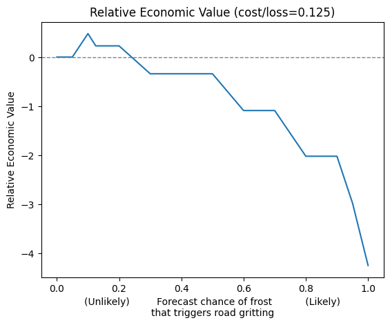
Remember that REV is the forecast value relative to perfect foreknowledge versus acting on climatological information. From earlier, for this particular cost/loss ratio, acting on climatological information would mean gritting every night.
In the above graph, the far left hand side shows every forecast is triggering the user to grit the roads, which is the same as the fall-back (climatological) strategy without forecasts, so REV = 0. On the far right hand side of the graph, none of the forecasts trigger action and so:
In this particular case, the highest REV happens at forecast probability threshold = 10%. Therefore, the optimal strategy for this user is to only grit the roads when the forecast is for >10% chance of frost. This may seem cautious but this is due to the low cost of protecting relative to the high cost of a missed event. Furthermore, the optimal probability threshold (10%) is different from the cost-loss ratio (0.125) because the forecasts are not perfectly calibrated.
Visualizing the Economic Value Curve#
So far, we have been considering one particular decision-maker but we can generalise the problem to consider a range of decision-makers. For example, commercial horticulture might deploy expensive heaters, airports may engage in de-icing, community services may check on vulnerable populations and so on. Each sector would have a different cost-loss ratio, particular to their decision-making context.
First, start with a case in which the decision has been made (perhaps by the forecast producer) that any forecast of > 40% chance of frost will go out as a warning that frost will occur. Forecasts of < 40% chance will signal no frost. Then we calculate REV for a wide range of possible decision-makers. For simplicity, highly negative values are not shown.
In this example, we omit cost_loss_ratios as an input. As a default, it evaluates it at each percentile 0.01, 0.02 … 0.98, 0.99.
[6]:
rev_many_users = relative_economic_value(fcst_probabilistic,
                                         obs,
                                         probability_thresholds=[0.4]
                                         )

rev_many_users.plot.line(x='cost_loss_ratio', add_legend=False)

plt.title(f"Relative Economic Value")
plt.xlabel("Cost Loss Ratio")
plt.ylabel("Relative Economic Value")
plt.ylim(-0.1, 1)
plt.axhline(0, color='gray', linewidth=1, linestyle='--')
plt.xlim(0, 1)
plt.show()
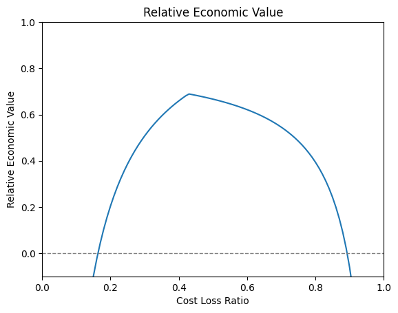
For users with a cost-loss of around 0.4-0.6, the forecasts are highly valuable. However, when the cost-loss is very low (left side of the graph), just a few missed events can mean catastrophic losses. On the right side, the cost of protection is so high that any false alarms would mean too high levels of waste. Therefore, users with very low/high cost-loss ratios should not rely on the forecasts but instead the rational behavior is to always/never protect (respectively).
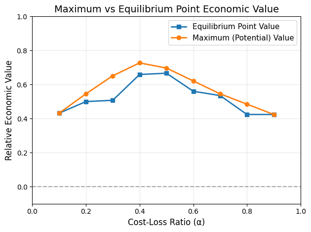
Derived Metrics: Equilibrium Point and Maximum Value#
When a user is unfamiliar with the performance of a particular forecasting system, it is often a good strategy to trust that the forecasts are probablistically reliable. In other words, when a forecast says there is a 80% chance of something happening, the event will happen 80% of the time, in the long run. This then becomes a special case where the user would use their particular cost-loss value as the forecast probability threshold to act upon. For example, with a cost-loss of 0.125, the user should act on the forecasts when it is 12.5% chance of the event or higher, and not act otherwise.
However, if a user does have knowledge of the forecasting system performance, they can choose the optimal forecast probability threshold which gives the highest economic value. For example, if a forecast was not necessarily reliable, the user with a cost-loss of 0.125 might find that a forecast probability threshold of 30% gives them the maximum value.
Therefore, we have the option of two derived metrics:
Equilibrium Point: REV when users set their decision threshold equal to their cost-loss ratio (assumes forecast probabilities are reliable)
Maximum value: The best REV achievable across all decision thresholds. Sometimes called the “potential value”.
[7]:
matching_values = np.linspace(0, 1, 10, endpoint=False)

# A requirement of "equilibrium_point" is that the cost_loss_ratios and probability threshold values match
rev_derived = relative_economic_value(
    fcst_probabilistic,
    obs,
    cost_loss_ratios=matching_values,
    probability_thresholds=matching_values,
    generate_maximum_rev = True,
    generate_equilibrium_point_rev = True,
)

print("REV for equilibrium point (using probability directly):\n")
print(rev_derived['equilibrium_point'])
print("\nMaximum REV at each cost-loss ratio:\n")
print(rev_derived['maximum'])

plt.plot(matching_values, rev_derived['equilibrium_point'],
        marker='s', linewidth=2, label='Equilibrium Point Value')
plt.plot(matching_values, rev_derived['maximum'],
        marker='o', linewidth=2, label='Maximum (Potential) Value')
plt.axhline(y=0, color='k', linestyle='--', alpha=0.3)
plt.xlabel('Cost-Loss Ratio (α)', fontsize=12)
plt.ylabel('Relative Economic Value', fontsize=12)
plt.title('Maximum vs Equilibrium Point Economic Value', fontsize=14)
plt.ylim(-0.1, 1)
plt.xlim(0, 1)

plt.legend(fontsize=11)
plt.grid(True, alpha=0.3)
plt.tight_layout()
plt.show()
REV for equilibrium point (using probability directly):

<xarray.DataArray 'equilibrium_point' (cost_loss_ratio: 10)> Size: 80B
array([       nan, 0.43181818, 0.5       , 0.50757576, 0.65909091,
       0.66666667, 0.56060606, 0.53535354, 0.42424242, 0.42424242])
Coordinates:
  * cost_loss_ratio        (cost_loss_ratio) float64 80B 0.0 0.1 0.2 ... 0.8 0.9
    probability_threshold  (cost_loss_ratio) float64 80B 0.0 0.1 0.2 ... 0.8 0.9

Maximum REV at each cost-loss ratio:

<xarray.DataArray 'maximum' (cost_loss_ratio: 10)> Size: 80B
array([       nan, 0.43181818, 0.54545455, 0.65151515, 0.72727273,
       0.6969697 , 0.62121212, 0.54545455, 0.48484848, 0.42424242])
Coordinates:
  * cost_loss_ratio        (cost_loss_ratio) float64 80B 0.0 0.1 0.2 ... 0.8 0.9
    probability_threshold  (cost_loss_ratio) float64 80B 0.0 0.1 0.2 ... 0.8 0.9
Working With Weights#
When evaluating forecasts over large spatial domains, simple averaging can be misleading. Grid cells near the poles represent smaller areas than cells near the equator, yet naive averaging treats them equally. Cosine weighting corrects this by applying weights proportional to cos(latitude), matching the actual surface area each grid cell represents.
This example shows weighting by latitude, but it is possible to weight by any dimension of the input data, such as time for particularly interesting events. The weights array only needs the dimensions you are weighting (here, just lat). Xarray broadcasts it automatically across time and lon dimensions, so you do not need to manually expand the weights to match the full forecast shape.
[8]:
fcst_lat30 = [1] * 5 + [0] * 5 + [1] * 10 + [0] * 80
obs_lat30 = [1] * 5 + [1] * 5 + [0] * 10 + [0] * 80

# Latitude 45°: Moderate skill (REV = 0.5)
fcst_lat45 = [1] * 7 + [0] * 3 + [1] * 8 + [0] * 82
obs_lat45 = [1] * 7 + [1] * 3 + [0] * 8 + [0] * 82

# Latitude 60°: Higher skill (REV = 0.75)
fcst_lat60 = [1] * 9 + [0] * 1 + [1] * 6 + [0] * 84
obs_lat60 = [1] * 9 + [1] * 1 + [0] * 6 + [0] * 84

# Stack into spatial arrays: (time, lat, lon)
fcst_data = np.array([fcst_lat30, fcst_lat45, fcst_lat60]).T[:, :, np.newaxis]
obs_data = np.array([obs_lat30, obs_lat45, obs_lat60]).T[:, :, np.newaxis]

fcst_spatial = xr.DataArray(
    fcst_data,
    dims=["time", "lat", "lon"],
    coords={"time": range(100), "lat": [30, 45, 60], "lon": [0]}
)

obs_spatial = xr.DataArray(
    obs_data,
    dims=["time", "lat", "lon"],
    coords={"time": range(100), "lat": [30, 45, 60], "lon": [0]}
)

# First, compute REV without weights (simple average)
rev_unweighted_by_lat = relative_economic_value(
    fcst_spatial,
    obs_spatial,
    cost_loss_ratios=[0.2],
    preserve_dims='lat'
)

rev_unweighted = relative_economic_value(
    fcst_spatial,
    obs_spatial,
    cost_loss_ratios=[0.2],
    reduce_dims='all'
)

lats = [30, 45, 60]

print("REV versus latitude (unweighted)):")
for lat, rev_value in zip(lats, rev_unweighted_by_lat.values):
    print(f"  {lat}°: {rev_value[0]:.4f}")

print(f"\nUnweighted REV: {rev_unweighted.values[0]:.3f}")

# Now apply cosine latitude weighting
# cos(latitude) gives each grid cell weight proportional to its actual surface area

weights = xr.DataArray(
    create_latitude_weights(lats),
    dims=["lat"],
    coords={"lat": lats}
)

print("\nLatitude weights:")
for lat, weight in zip(lats, weights.values):
    print(f"  {lat}°: {weight:.4f}")

rev_weighted = relative_economic_value(
    fcst_spatial,
    obs_spatial,
    cost_loss_ratios=[0.2],
    reduce_dims='all',
    weights=weights
)

print(f"\nWeighted REV: {rev_weighted.values[0]:.6f}")
REV versus latitude (unweighted)):
  30°: 0.2500
  45°: 0.5000
  60°: 0.7500

Unweighted REV: 0.500

Latitude weights:
  30°: 0.8660
  45°: 0.7071
  60°: 0.5000

Weighted REV: 0.455861
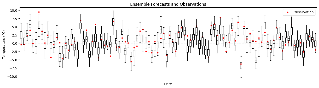
Working with Ensemble Forecasts#
Ensemble forecasts represent uncertainty through multiple members. We can convert ensembles to probabilities using binary_discretise_proportion, then evaluate their economic value.
[9]:
# Create a synthetic 50-member ensemble forecast for temperature
# Event of interest: temperature below 0°C (freezing)
n_times = 100
n_members = 50

#Latent true signal: seeds both obs and ensemble perturbations
seed_temps = np.random.normal(1, 3, n_times)

obs_temps = seed_temps + np.random.normal(0, 2, n_times)

ensemble = np.random.normal(
    seed_temps[:, np.newaxis],
    1.5,  # Ensemble spread
    (n_times, n_members)
)

ensemble_xr = xr.DataArray(
    ensemble,
    dims=["time", "member"],
    coords={
        "time": np.arange(n_times),
        "member": np.arange(n_members)
    }
)

# Observations
obs_xr = xr.DataArray(
    obs_temps,
    dims=["time"],
    coords={"time": np.arange(n_times)}
)

times = ensemble_xr["time"].values
ensemble_values = ensemble_xr.values

fig, ax = plt.subplots(figsize=(16, 4))

ax.boxplot(
    ensemble_values.T,
    positions=times,
    widths=0.6,
    showfliers=False,
    medianprops=dict(color='black', linewidth=0.5),  # invisible
)

ax.scatter(times, obs_xr.values, color="red", s=10, label="Observation")

ax.set_xlabel("Date")
ax.set_xticks([])
ax.set_ylabel("Temperature (°C)")
ax.set_title("Ensemble Forecasts and Observations")
ax.axhline(y=0, color='k', linestyle='--', alpha=0.3)
ax.legend()
plt.show()
[10]:
# Convert ensemble to probability of freezing using binary_discretise_proportion
prob_freezing = binary_discretise_proportion(
ensemble_xr,
thresholds=[0], # Event threshold: temperature < 0°C
mode='<',
reduce_dims=['member'] # Calculate proportion across ensemble members
)
# Rename dimension to avoid conflict with REV's threshold parameter
prob_freezing = prob_freezing.rename({'threshold': 'event_threshold'})
# Extract probability for 0°C threshold
prob_freezing_0c = prob_freezing.sel(event_threshold=0, drop=True)
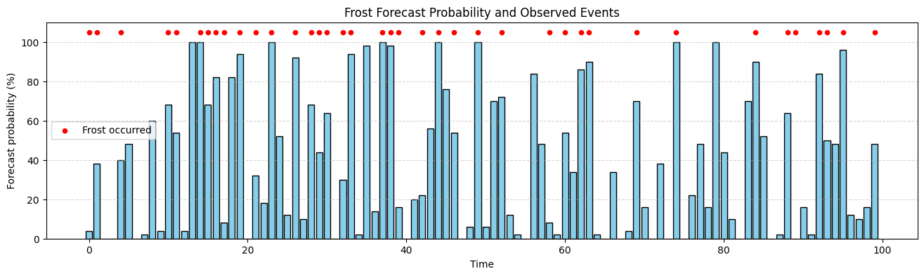
print("Forecast chance of frost")
print(prob_freezing_0c)
# Convert observations to binary: did it freeze (1) or not (0)?
obs_freezing_0c = (obs_xr < 0).astype(int)
print("Observed frost instances")
print(obs_freezing_0c)
fig, ax = plt.subplots(figsize=(16, 4))
ax.bar(times, prob_freezing_0c.values* 100, color="skyblue", edgecolor="black")
# Overlay observations as dots at the top of the chart
y_top = 105 # a bit above 100%
ax.scatter(times[obs_freezing_0c.values == 1], np.full(obs_freezing_0c.values.sum(), y_top),
color="red", s=20, label="Frost occurred")
# Labels and styling
ax.set_xlabel("Time")
ax.set_ylabel("Forecast probability (%)")
ax.set_ylim(0, 110)
ax.set_title("Frost Forecast Probability and Observed Events")
ax.legend()
ax.grid(True, axis='y', linestyle='--', alpha=0.5)
Forecast chance of frost
<xarray.DataArray (time: 100)> Size: 800B
array([0.04, 0.38, 0.  , 0.  , 0.4 , 0.48, 0.  , 0.02, 0.6 , 0.04, 0.68,
       0.54, 0.04, 1.  , 1.  , 0.68, 0.82, 0.08, 0.82, 0.94, 0.  , 0.32,
       0.18, 1.  , 0.52, 0.12, 0.92, 0.1 , 0.68, 0.44, 0.64, 0.  , 0.3 ,
       0.94, 0.02, 0.98, 0.14, 1.  , 0.98, 0.16, 0.  , 0.2 , 0.22, 0.56,
       1.  , 0.76, 0.54, 0.  , 0.06, 1.  , 0.06, 0.7 , 0.72, 0.12, 0.02,
       0.  , 0.84, 0.48, 0.08, 0.02, 0.54, 0.34, 0.86, 0.9 , 0.02, 0.  ,
       0.34, 0.  , 0.04, 0.7 , 0.16, 0.  , 0.38, 0.  , 1.  , 0.  , 0.22,
       0.48, 0.16, 1.  , 0.44, 0.1 , 0.  , 0.7 , 0.9 , 0.52, 0.  , 0.02,
       0.64, 0.  , 0.16, 0.02, 0.84, 0.5 , 0.48, 0.96, 0.12, 0.1 , 0.16,
       0.48])
Coordinates:
  * time     (time) int64 800B 0 1 2 3 4 5 6 7 8 ... 91 92 93 94 95 96 97 98 99
Attributes:
    discretisation_tolerance:  0
    discretisation_mode:       <
Observed frost instances
<xarray.DataArray (time: 100)> Size: 800B
array([1, 1, 0, 0, 1, 0, 0, 0, 0, 0, 1, 1, 0, 0, 1, 1, 1, 1, 0, 1, 0, 1,
       0, 1, 0, 0, 1, 0, 1, 1, 1, 0, 1, 1, 0, 0, 0, 1, 1, 1, 0, 0, 1, 0,
       1, 0, 1, 0, 0, 1, 0, 0, 1, 0, 0, 0, 0, 0, 1, 0, 1, 0, 1, 1, 0, 0,
       0, 0, 0, 1, 0, 0, 0, 0, 1, 0, 0, 0, 0, 0, 0, 0, 0, 0, 1, 0, 0, 0,
       1, 1, 0, 0, 1, 1, 0, 1, 0, 0, 0, 1])
Coordinates:
  * time     (time) int64 800B 0 1 2 3 4 5 6 7 8 ... 91 92 93 94 95 96 97 98 99
[11]:
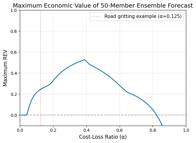
# Now calculate REV using these ensemble-derived probabilities
matching_values = np.linspace(0, 1, 100, endpoint=False)

rev_ensemble = relative_economic_value(
    prob_freezing_0c,
    obs_freezing_0c,
    cost_loss_ratios=matching_values,
    probability_thresholds=matching_values,
    generate_maximum_rev = True
)

# Plot
plt.plot(matching_values , rev_ensemble['maximum'], linewidth=2)
plt.axhline(y=0, color='k', linestyle='--', alpha=0.3)
plt.axvline(x=0.125, color='red', linestyle=':', alpha=0.5,
           label='Road gritting example (α=0.125)')
plt.xlabel('Cost-Loss Ratio (α)', fontsize=12)
plt.ylabel('Maximum REV', fontsize=12)
plt.title('Maximum Economic Value of 50-Member Ensemble Forecast', fontsize=14)
plt.legend(fontsize=11)
plt.grid(True, alpha=0.3)
plt.xlim(0, 1)
plt.ylim(-0.1, 1)
plt.tight_layout()
plt.show()
Working with Multiple Dimensions#
REV can preserve spatial or other dimensions while aggregating over time.
[12]:
# Create forecast with spatial dimension (e.g., different road segments)
n_locations = 5
n_days = 100

fcst_spatial = xr.DataArray(
    np.random.uniform(0, 1, (n_days, n_locations)),
    dims=['time', 'location'],
    coords={
        'time': np.arange(n_days),
        'location': ['Route_A', 'Route_B', 'Route_C', 'Route_D', 'Route_E']
    }
)

# Different base rates for different locations
base_rates = np.array([0.1, 0.15, 0.25, 0.3, 0.6])
obs_spatial = xr.DataArray(
    np.random.binomial(1, base_rates + 0.3 * fcst_spatial.values, (n_days, n_locations)),
    dims=['time', 'location'],
    coords={'time': np.arange(n_days), 'location': fcst_spatial.location}
)

# Calculate REV, preserving location dimension
rev_spatial = relative_economic_value(
    fcst_spatial,
    obs_spatial,
    cost_loss_ratios=[0.1],
    probability_thresholds=[0.1, 0.2, 0.3],
    reduce_dims=['time'],  # Aggregate over time, preserve location
)

print("REV at each location:")
print(rev_spatial.to_dataframe("REV").unstack("probability_threshold"))

# Reducing the time dimension is the same as preserving the location dimension.
# You cannot specify preserve_dims and reduce_dims at the same time.
rev_preserve_dim = relative_economic_value(
    fcst_spatial,
    obs_spatial,
    cost_loss_ratios=[0.1],
    probability_thresholds=[0.1, 0.2, 0.3],
    preserve_dims=['location'],
)

if rev_preserve_dim.equals(rev_spatial):
    print("\nPreserving dimensions and reducing dimensions are two ways of achieving the same result.")
REV at each location:
                               REV
probability_threshold          0.1       0.2       0.3
location cost_loss_ratio
Route_A  0.1             -0.012048  0.024096  0.180723
Route_B  0.1             -0.394737 -0.342105 -0.289474
Route_C  0.1             -0.491525 -0.966102 -1.372881
Route_D  0.1             -0.177419 -0.064516 -0.516129
Route_E  0.1             -1.750000 -4.821429 -5.642857

Preserving dimensions and reducing dimensions are two ways of achieving the same result.
Working with Datasets#
REV can work with Xarray datasets.
[13]:
# Forecasts can be datasets
fcst_ds = xr.Dataset(
    {"ecmwf": xr.DataArray([0, 1, 1, 0], dims=["time"]), "access": xr.DataArray([1, 0, 1, 1], dims=["time"])}
    )

obs = xr.DataArray([0, 1, 0, 1], dims=["time"])

result = relative_economic_value(fcst_ds, obs, cost_loss_ratios = [0.5])

print(result)

# Observations can also be datasets
fcst = xr.DataArray([0.2, 0.8, 0.6, 0.4], dims=["time"])
obs_ds = xr.Dataset(
        {
            "station_data": xr.DataArray([0, 1, 1, 0], dims=["time"]),
            "radar_data": xr.DataArray([0, 0, 1, 0], dims=["time"]),
        }
    )

result = relative_economic_value(fcst, obs_ds, cost_loss_ratios = [0.3, 0.7], probability_thresholds=[0.5])

print(result)

# It is also possible to make both observations and forecasts datasets although the
# output names are changed.

result = relative_economic_value(fcst_ds, obs_ds, cost_loss_ratios = [0.3, 0.7], probability_thresholds=[0.5])
print(result)
<xarray.Dataset> Size: 24B
Dimensions:          (cost_loss_ratio: 1)
Coordinates:
  * cost_loss_ratio  (cost_loss_ratio) float64 8B 0.5
Data variables:
    ecmwf            (cost_loss_ratio) float64 8B 0.0
    access           (cost_loss_ratio) float64 8B -0.5
<xarray.Dataset> Size: 56B
Dimensions:                (probability_threshold: 1, cost_loss_ratio: 2)
Coordinates:
  * probability_threshold  (probability_threshold) float64 8B 0.5
  * cost_loss_ratio        (cost_loss_ratio) float64 16B 0.3 0.7
Data variables:
    station_data           (probability_threshold, cost_loss_ratio) float64 16B ...
    radar_data             (probability_threshold, cost_loss_ratio) float64 16B ...
<xarray.Dataset> Size: 88B
Dimensions:                   (probability_threshold: 1, cost_loss_ratio: 2)
Coordinates:
  * probability_threshold     (probability_threshold) float64 8B 0.5
  * cost_loss_ratio           (cost_loss_ratio) float64 16B 0.3 0.7
Data variables:
    access__vs__radar_data    (probability_threshold, cost_loss_ratio) float64 16B ...
    access__vs__station_data  (probability_threshold, cost_loss_ratio) float64 16B ...
    ecmwf__vs__radar_data     (probability_threshold, cost_loss_ratio) float64 16B ...
    ecmwf__vs__station_data   (probability_threshold, cost_loss_ratio) float64 16B ...
Custom Dimension Names and Extracting Particular Thresholds#
You can customize the output dimension names to avoid conflicts. You can also output a subset of your selected probability thresholds.
[14]:
rev_custom = relative_economic_value(
    fcst_spatial,
    obs_spatial,
    cost_loss_ratios=[0.1, 0.3, 0.5],
    probability_thresholds=[0.1, 0.2, 0.4, 0.6],
    probability_threshold_dim='decision_threshold',
    cost_loss_dim='alpha'
)

print("REV with custom dimension names:")
print(rev_custom)

rev_subset = relative_economic_value(
    fcst_spatial,
    obs_spatial,
    cost_loss_ratios=[0.1, 0.3, 0.5],
    probability_thresholds=[0.1, 0.2, 0.4, 0.6],
    probability_threshold_outputs=[0.1, 0.6],
)

print("\n\nREV with a subset of output thresholds:")
print(rev_subset)
REV with custom dimension names:
<xarray.DataArray (decision_threshold: 4, alpha: 3)> Size: 96B
array([[-0.38961039, -0.02164502, -0.52083333],
       [-0.71428571, -0.02164502, -0.41666667],
       [-1.37337662, -0.00974026, -0.18229167],
       [-2.3538961 , -0.10281385, -0.046875  ]])
Coordinates:
  * decision_threshold  (decision_threshold) float64 32B 0.1 0.2 0.4 0.6
  * alpha               (alpha) float64 24B 0.1 0.3 0.5


REV with a subset of output thresholds:
<xarray.Dataset> Size: 72B
Dimensions:          (cost_loss_ratio: 3)
Coordinates:
  * cost_loss_ratio  (cost_loss_ratio) float64 24B 0.1 0.3 0.5
Data variables:
    threshold_0_1    (cost_loss_ratio) float64 24B -0.3896 -0.02165 -0.5208
    threshold_0_6    (cost_loss_ratio) float64 24B -2.354 -0.1028 -0.04688
Things to try next#
The REV score uses the probability of detection and false alarm rate in its calculations. These are used in the ROC score. See the ROC tutorial and construct an example where both ROC and REV are calculated on the same dataset.
To better understand the “equilibrium point” outputs, created forecasts that are probabilistically reliable, and then create forecasts are biased. See how the results for the equilibrium and the maximum potential value REV differ for these two forecasting systems.
Explore the effects of ensemble size on economic value. Create a large ensemble (e.g. 500 members) and the progressively thin (sub-sample) the ensemble (100, 50, 25, 10, 5 members) and see how value changes, if at all.
Create two forecast systems: one that is well-calibrated (probabilistically reliable) but conservative, and another that is poorly calibrated but aggressive in its warnings. Compare their Brier Scores and REV across different cost-loss ratios. Can you find scenarios where the “worse” forecast (by Brier Score) delivers higher economic value? What does this reveal about optimizing for accuracy versus optimizing for decision-making?
References#
Murphy, A. H. (1977). The value of climatological, categorical and probabilistic forecasts in the cost-loss ratio situation. Monthly Weather Review, 105(7), 803-816.
Richardson, D. S. (2000). Skill and relative economic value of the ECMWF ensemble prediction system. Quarterly Journal of the Royal Meteorological Society, 126(563), 649-667.
Roulin, E. (2007). Skill and relative economic value of medium-range hydrological ensemble predictions. Hydrology and Earth System Sciences, 11(2), 725-737.
Thornes, J. E., & Stephenson, D. B. (2001). How to judge the quality and value of weather forecast products. Meteorological Applications, 8(3), 307-314.
Thornes, J. E. (2002, January). The Quality and Value of Road Weather Forecast. In The Proceedings of The 11th. PIARC International Winter Road Congress. (https://proceedings-sapporo2002.piarc.org/en/pdf/doc_pdf/communications/V58e.pdf)
Zhu, Y., Toth, Z., Wobus, R., Richardson, D., & Mylne, K. (2002). The economic value of ensemble-based weather forecasts. Bulletin of the American Meteorological Society, 83(1), 73-84.